Evaluate Bezière curve

One of the tasks for the coming release of OpenPatrician is a better representation of the price development of wares with respect to the amount that is available. The idea is to define the curve visually and then transform the parameters of the curve into a formula that allows the computation of the price of the ware, given an available amount.
A natural choice for that is to define the curve as a Bezière curve with is very intuitive to tweak until the curve looks the way you want.

The more tricky part is to translate these information into a workable formula. The type of the Bezière curve that I have in mind is a cubic curve, witch means four set of control points, where the first and the last one define the start respectively end of the curve and the other two the tangential direction of the curve going out of the start point respectively coming into the end point.

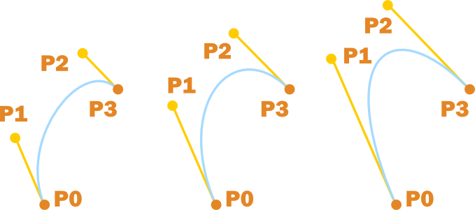
A good starting point to learn more about Bezièr curves is the article from which I have taken the above image, then of course Wikipedia and a Bezièr primer. As it turns out the curve can be described by this mathematical function:

Where t is on the interval [0,1] representing a point on the curve, with the interval [0,1] representing the whole length of the curve. When resolving this you get two formulas:

x(t) = x¹ * (1-t)₃ + x² * 3(1-t)₂*t + x³*3(1-t)*t₂ + x⁴*t₃

y(t) = y¹ * (1-t)₃ + y² * 3 (1-t)₂*t + y³*3(1-t)*t₂ + y⁴*t₃

This leaves us with two equations with 3 unknowns. As you might know this is not enough to resolve the formula in a mathematical sense (you would need one more formula in addition).

However when looking at the problem at hand it is possible to find an acceptable solution. This is not general purpose but might give you some idea how to approach a similar situation. First there are several restrictions and/or assumptions that hold for my specific problem.

1. The curve itself is not folded in itself but it is continuously decreasing: y(x+?) ? y(x), where ? is the smallest positive number.
2. The curve is not folded (does not have cusp or loops).
3. The only interesting points are for whole numbered x values.
4. The y value at position x can be rounded to the next whole number.
5. The curve itself is not dynamic, meaning it does not change from one call to the other. It is only defined by static parameters.

Especially the last point gives a possible approach, as once a value that is computed once can be reused again. Together with the fact that there are a numbered amount of points in the range of the curve between x¹ and x⁴, all these points can be calculated on first use and then cached.

Now how do we do this? Simply by taking the above formula for x(t) and evaluate it  for certain values of t, and check if the resulting value x is close enough to the next whole number. Then we can calculate y(t) for the same value of t.

So let’s take a look at how to calculate a point for a given value of t (The algorithm is the same as in the aforementioned article, only adapted to 2D in Java):

/**
 * Calculate the point (x,y-coordinates) on the bezier curve defined by the four control points for
 * parameter <code>t</code>
 * @param t Value in the range [0,1] defining the fragment length on the curve.
 * @param start control point marking the start of the curve
 * @param cp1 first control point defining the tangential direction of the curve leaving <code>start</code>
 * @param cp2 second control point defining the tangential direction of the curve going into <code>end</code>
 * @param end control point marking the end of the curve.
 * @return Point (x,y-coordinates) at position <code>t</code> on the curve.
 */
public Point2D caclulateBezierPoint(double t, Point2D start, Point2D cp1, Point2D cp2, Point2D end) {
    // B(t) = (1-t)³*start + 3*(1-t)²*t*cp1 + 3*(1-t)*t²*cp2 + t³*end
    double u = 1 - t;
    double tSquare = t*t;
    double tQube = t*t*t;
    double uSquare = u*u;
    double uQube = u*u*u;

    Point2D summand1 = start.multiply(uQube); // (1-t)³*start
    Point2D summand2 = cp1.multiply(3 * uSquare * t); // 3*(1-t)²*t*cp1
    Point2D summand3 = cp2.multiply(3 * u * tSquare); // 3*(1-t)*t²*cp2
    Point2D summand4 = end.multiply(tQube); // t³*end
    return summand1.add(summand2).add(summand3).add(summand4);
}

There is nothing special to that code, simply implementing the mentioned formula.

For the calculating all the points of interest (every x that is a whole number between x¹ and x⁴): There are two parameters (? and ?) that must be considered:

1. ?: How close is close enough to consider x to be approximately equal to the next whole number. I have chosen a value of 0.1 as the value of y for that x is also rounded to then nearest whole number. However this parameter is dependent on the second parameter and the incline of the curve: if the incline is shallow it might be that there is no evaluation of the formula for t so that x(t+?) ? n and x(t+?-?) ? n, where n is the whole number.
2. ?: This is the step size with which the value t is increased. Imagine the most simple curve, a straight line from start to end, then a good measure would be the difference between x(end) and x(start), which is the number of points in between. However the curve is probably a bit longer than a direct horizontal line. Therefore more points are required. To compensate for the possibility of a shallow curve I chose a factor of 0.1, which can be roughly interpreted that there should be about ten iteration steps of t before hitting the next whole number.

With that in mind this calculation makes more sense:

/**
 * Calculate a list of points at discrete x coordinates.<br>
 * PRE: The bezier curve does not bend back on itself.
 * @param start control point marking the start of the curve
 * @param cp1 first control point defining the tangential direction of the curve leaving <code>start</code>
 * @param cp2 second control point defining the tangential direction of the curve going into <code>end</code>
 * @param end control point marking the end of the curve.
 * @return List of points for x coordinates from start to end.
 */
public List<Point2D> calculateDiscreteBezierPoints(Point2D start, Point2D cp1, Point2D cp2, Point2D end) {
    Preconditions.checkArgument(end.getX() > start.getX(), "The x coordinate of the end point must be larger than the one of the start point");
    int nbPoints = (int) Math.rint(end.getX() - start.getX());
    double delta = 0.1/nbPoints; // step size of t
    double epsilon = 0.1; // stop criterium when found point's x value is assumed accurate enough
    List<Point2D> points = new ArrayList<>(nbPoints);
    double lastX = start.getX() - 1;
    double t;
    for (t = 0; t <= 1; t += delta) {
        Point2D nextPoint = caclulateBezierPoint(t, start, cp1, cp2, end);
        if (nextPoint.getX() > lastX + 0.5) {
            double descreteX = (int)Math.rint(nextPoint.getX());
            if (Math.abs(descreteX - nextPoint.getX()) < epsilon) { // if the distance between the next integer and x is smaller than epsilon
                lastX = nextPoint.getX();
                Point2D p = new Point2D(Math.rint(nextPoint.getX()), Math.rint(nextPoint.getY()));
                points.add(p);
            }
        }
    }
    if (points.size() == nbPoints) { // last point is missing
        points.add(end);
    }
    return points;
}

There are two issues in the code that need some further explanation:

The use of lastX is in there to determine that once we have found a value that we consider close enough to a whole number, we can ignore other values that are equally close until we are nearing the next whole number: If lastX has a value of 43.94, then we do not need to investigate x(t) values that are nearer to 43 than to 44.

The other thing is that we add the last point at the end. In all probably the last value of t evaluated is < 1, which means that the end point is not part of the list, which it should be.